A forest has many more components than the data have effects: every
set of predictors that some tree splits on gives one, and with enough
splits nearly every set does. Most of them are tiny and fit noise. By
default rpf() prunes them, so that the model it returns has
the few components worth reading, and predicts better.
The data: two main effects, a two-way and a three-way interaction;
x5 has no effect.
make_data <- function(n) {
  d <- data.frame(matrix(runif(n * 5, -1, 1), ncol = 5, dimnames = list(NULL, paste0("x", 1:5))))
  d$y <- sin(pi * d$x1) + d$x2 + 2 * d$x1 * d$x3 + 3 * d$x2 * d$x3 * d$x4 + rnorm(n, sd = 0.3)
  d
}
set.seed(3)
train <- make_data(1000)
test <- make_data(2000)
The forest and the pruned model
prune = FALSE returns the forest itself.
prune_components() prunes a forest, and with its defaults
it gives exactly the model that the default rpf() call
returns from the same random number state:
set.seed(10)
forest <- rpf(y ~ ., data = train, prune = FALSE, nthreads = 2)
pruned <- prune_components(forest, train)

set.seed(10)
identical(predict(pruned, test), predict(rpf(y ~ ., data = train, nthreads = 2), test))
#> [1] TRUE
The pruned model does not hold the forest it was pruned from
(keep_forest = TRUE keeps it, in rpf() and in
prune_components()). To try other settings, prune the
forest again, as below.
The forest has 25 nonzero components; the pruned model keeps 4:
rmse <- function(m) sqrt(mean((test$y - predict(m, test)$.pred)^2))
c(forest = rmse(forest), pruned = rmse(pruned))
#>    forest    pruned
#> 0.5201452 0.3416975
Often, the pruned model is both smaller and more accurate on new data.
What is left out, and why
Every component f_S of the forest has a size: its share
of the variance of the forest’s prediction on the training rows,
Var(f_S) / Var(f). A component is kept if its share is at
least a threshold tau. The forest’s components, largest
first (pruned$display$first is the model before the display
step, below):
first <- pruned$display$first
head(first$components[order(-first$components$share), c("component", "share", "kept")], 10)
#>    component        share  kept
#> 1         x1 0.3473664391  TRUE
#> 7      x1:x3 0.2868914361  TRUE
#> 2         x2 0.2112874391  TRUE
#> 22  x2:x3:x4 0.0251899829  TRUE
#> 10     x2:x3 0.0029453603 FALSE
#> 3         x3 0.0020258604 FALSE
#> 6      x1:x2 0.0018023100 FALSE
#> 16  x1:x2:x3 0.0014639326 FALSE
#> 11     x2:x4 0.0008721929 FALSE
#> 8      x1:x4 0.0008204013 FALSE
Two rules are compared:
- D (drop): the prediction is the intercept plus the kept components, as the forest has them.
- R (drop and refit): one coefficient per kept component and a new intercept, fitted by least squares on the kept components. The components keep their shape and change their scale. This undoes the forest’s shrinkage of interactions, which comes from averaging families of which some never find a given interaction.
The candidates are both rules at eight thresholds, tau =
0, 0.01%, 0.03%, 0.1%, 0.3%, 1%, 3% and 10%.
The choice, out of bag
Each candidate is scored by its out-of-bag error: every family’s components are evaluated at the training rows outside its bootstrap sample, so the score uses no refit of the forest. The coefficients of rule R are fitted on these out-of-bag components too, because the forest’s own components have fitted the noise of the training rows, and least squares on them would scale the components up.
The choice is the largest tau whose error is within one
standard error of the lowest (select = "1se"), and at that
tau the rule with the lower error:
first$oob[, c("rule", "tau", "oob_rmse", "se_mse", "n_kept", "min", "one_se")]
#>    rule   tau  oob_rmse      se_mse n_kept   min one_se
#> 1     D 0e+00 0.5233229 0.009598275     25 FALSE  FALSE
#> 2     D 1e-04 0.5229136 0.009899163     20 FALSE  FALSE
#> 3     D 3e-04 0.5207291 0.010147910     17 FALSE  FALSE
#> 4     D 1e-03 0.5179311 0.007072532      8 FALSE  FALSE
#> 5     D 3e-03 0.5065508 0.008089898      4 FALSE  FALSE
#> 6     D 1e-02 0.5065508 0.008089898      4 FALSE  FALSE
#> 7     D 3e-02 0.6575630 0.018986193      3 FALSE  FALSE
#> 8     D 1e-01 0.6575630 0.018986193      3 FALSE  FALSE
#> 9     R 0e+00 0.3460312 0.002919835     25 FALSE  FALSE
#> 10    R 1e-04 0.3458509 0.003660649     20 FALSE  FALSE
#> 11    R 3e-04 0.3455838 0.003536658     17 FALSE  FALSE
#> 12    R 1e-03 0.3433686 0.003065870      8  TRUE  FALSE
#> 13    R 3e-03 0.3436807 0.003057481      4 FALSE  FALSE
#> 14    R 1e-02 0.3436807 0.003057481      4 FALSE   TRUE
#> 15    R 3e-02 0.6574524 0.020011210      3 FALSE  FALSE
#> 16    R 1e-01 0.6574524 0.020011210      3 FALSE  FALSE
tab <- first$oob
x <- seq_along(unique(tab$tau))
plot(NULL, xlim = range(x), ylim = range(tab$oob_rmse), xaxt = "n",
     xlab = "tau", ylab = "corrected OOB RMSE")
axis(1, at = x, labels = format(unique(tab$tau), scientific = FALSE, drop0trailing = TRUE),
     cex.axis = 0.8)
for (r in c("D", "R")) {
  s <- tab[tab$rule == r, ]
  lines(x, s$oob_rmse, type = "b", pch = 20, lty = if (r == "D") 2 else 1)
}
chosen <- tab[tab$one_se, ]
points(match(chosen$tau, unique(tab$tau)), chosen$oob_rmse, pch = 1, cex = 2, col = "orange", lwd = 2)
legend("topleft", c("rule D", "rule R", "chosen"), lty = c(2, 1, NA), pch = c(20, 20, 1),
       col = c("black", "black", "orange"), bty = "n")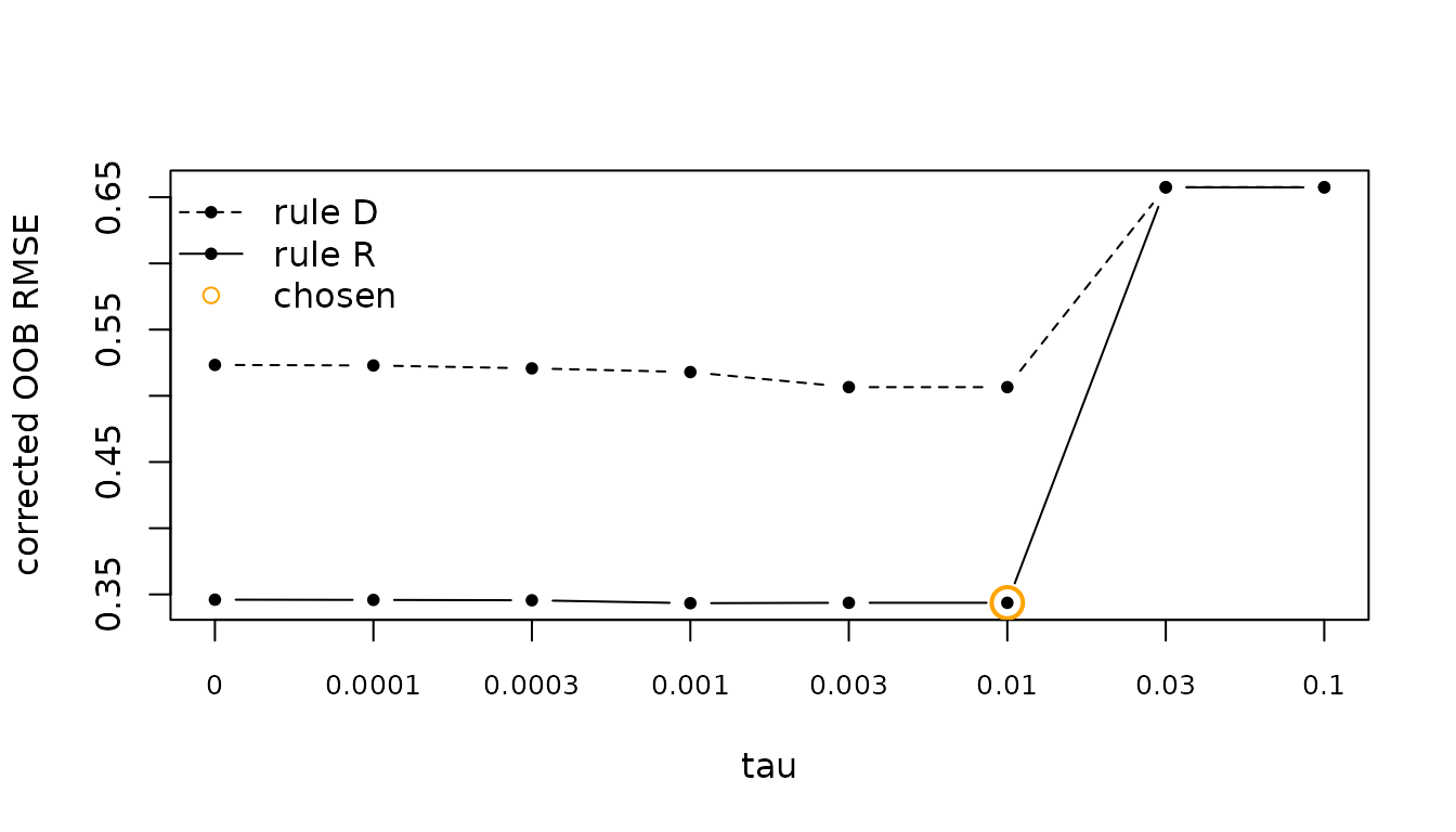
Here rule R’s refit lowers the error far below rule D’s at every
threshold that keeps the four true components. Under rule R the error
changes little over a wide range of tau, so the 1-SE rule
can take a large threshold and a small model.
select = "min" takes the lowest error instead, which keeps
more small components.
Note that it can happen that pruning drops a small true component if its fitted signal is not strong enough.
Other choices
prune_components() takes the candidates and the way of
choosing as arguments. A given rule and threshold are applied without a
choice:
given <- prune_components(forest, train, rule = "D", tau = 0.01)
given$components$component[given$components$kept]
#> [1] "x1"       "x2"       "x1:x3"    "x2:x3:x4"
select = "min" takes the lowest out-of-bag error:
sum(prune_components(forest, train, select = "min")$components$kept)
#> [1] 4
select_by = "cv" scores the candidates by K-fold
cross-validation instead, refitting the forest on each fold, so it costs
K more fits.
Often out-of-bag and cross-validation choose the same rule and threshold, the former with lower cost, but not always.
set.seed(10)
forest50 <- rpf(y ~ ., data = train, n_families = 50, prune = FALSE, nthreads = 2)
by_cv <- prune_components(forest50, train, select_by = "cv", seed = 1)
by_cv$cv[by_cv$cv$one_se, c("rule", "tau", "cv_rmse", "n_kept")]
#>    rule  tau   cv_rmse n_kept
#> 14    R 0.01 0.3611284      4
The display: components of three predictors
A component of three predictors is shown as heat maps over two of
them, one per interval of the third, and its own cut points can need
hundreds of heat maps. After the first pruning, every kept component of
three or more predictors that needs more than max_panels
(10) heat maps is coarsened:
- two of its predictors stay at full resolution;
- the others are cut into intervals with equal numbers of training
rows, at most
max_panelscells in all, and the component is averaged within each cell; - of all such forms, the one that keeps most of the component’s variance is taken.
Then the model is pruned again, by the same rule, with the coarsened components in place, so that the pruning judges the model that is shown and predicts. Often this gives a slightly lower test error than coarsening after pruning, or not coarsening at all.
pruned$display$forms
#>   component order      form forest_panels heat_maps  var_kept
#> 1  x2:x3:x4     3 coarsened           978        10 0.9935583
max_panels = Inf (in rpf() or
prune_components()) skips this step, and Reading the model shows how to read a
coarsened component.
The forest itself: prune = FALSE
With prune = FALSE, rpf() returns the
forest, of class rpf. Its predict_components()
gives every component, after purifying the forest on first use:
ncol(predict_components(forest, test)$m)
#> [1] 25
This is the place to start for your own pruning rule, or to look at components that the default leaves out.