Classification

For a factor outcome (binary or multi-class with more than two classes), rpf() fits a classification model. It takes the same steps as for regression, with the same defaults: the number of splits is chosen out of bag, the components are pruned, and three-way components are simplified such that each can be shown as the sum of at most 10 heat maps. The model predicts scores, and every score is a sum of components, as the prediction of a regression model is. With the losses "logit" (the default) and "exponential", the scores are on the log-odds scale: with two classes there is one score, the log-odds of the second class, and with more classes there is one score per class, and the scores sum to 0. With "L1" and "L2" the scores are not log-odds but fitted 0/1 class indicators. The losses are described in “The losses” below.

library(randomPlantedForest)
library(glex)

penguins <- na.omit(palmerpenguins::penguins)

Two classes

set.seed(1)
by_sex <- rpf(sex ~ ., data = penguins, nthreads = 2)
by_sex
#> ── Random Planted Forest model ─────────────────────────────────────────────────
#> Classification (logit loss), 2 classes: female, male. Scores = intercept + the sum of 4 components.
#> Intercept: 0.0746385
#> 
#> Components (largest first), importance = share of the variance of the prediction on the training rows:
#>  component      importance
#>  body_mass_g    55%       
#>  bill_depth_mm  37%       
#>  bill_length_mm 17%       
#>  species        14%       
#> 
#> How it was chosen:
#>   The forest: 200 tree families of 59 splits (chosen out of bag; growing stopped at 59).
#>   From the forest's 63 nonzero components (purified): those with a share of at least 3% of the forest's Var(prediction), as they are (rule D).
#>   Rule and threshold chosen by out-of-bag error (1-SE rule; 5 folds, seed 682372961) among 16 candidates.
#>   Left out: 59 components, shares together 4% (largest flipper_length_mm, 1.4%).

predict() returns probabilities by default, classes with type = "class", and the scores with type = "link":

predict(by_sex, head(penguins))
#> # A tibble: 6 × 2
#>   .pred_female .pred_male
#>          <dbl>      <dbl>
#> 1        0.152      0.848
#> 2        0.551      0.449
#> 3        0.768      0.232
#> 4        0.630      0.370
#> 5        0.121      0.879
#> 6        0.830      0.170
predict(by_sex, head(penguins), type = "class")
#> # A tibble: 6 × 1
#>   .pred_class
#>   <fct>      
#> 1 male       
#> 2 female     
#> 3 female     
#> 4 female     
#> 5 male       
#> 6 female
predict(by_sex, head(penguins), type = "link")
#> # A tibble: 6 × 1
#>    .pred
#>    <dbl>
#> 1  1.72 
#> 2 -0.205
#> 3 -1.20 
#> 4 -0.532
#> 5  1.99 
#> 6 -1.58

The components, on the scale of the scores

The components add up to the scores, not to the probabilities:

comp <- predict_components(by_sex, penguins)
head(comp$m)
#>    bill_length_mm bill_depth_mm body_mass_g  species
#>             <num>         <num>       <num>    <num>
#> 1:    -0.58025340     1.7503844  -0.7566046 1.234439
#> 2:    -0.52391729    -0.4248011  -0.5651751 1.234439
#> 3:    -0.09361972     0.4104165  -2.8233288 1.234439
#> 4:    -1.83280502     2.5005622  -2.5086987 1.234439
#> 5:    -0.52168263     2.9404168  -1.7410431 1.234439
#> 6:    -0.69556179    -0.2929853  -1.9051425 1.234439
all.equal(comp$intercept + rowSums(comp$m), predict(by_sex, penguins, type = "link")$.pred)
#> [1] TRUE

With two classes there is one score, the log-odds of the second level of the outcome (here male): a positive contribution moves a penguin towards male, a negative one towards female. glex draws them as for regression:

plot(comp, "body_mass_g")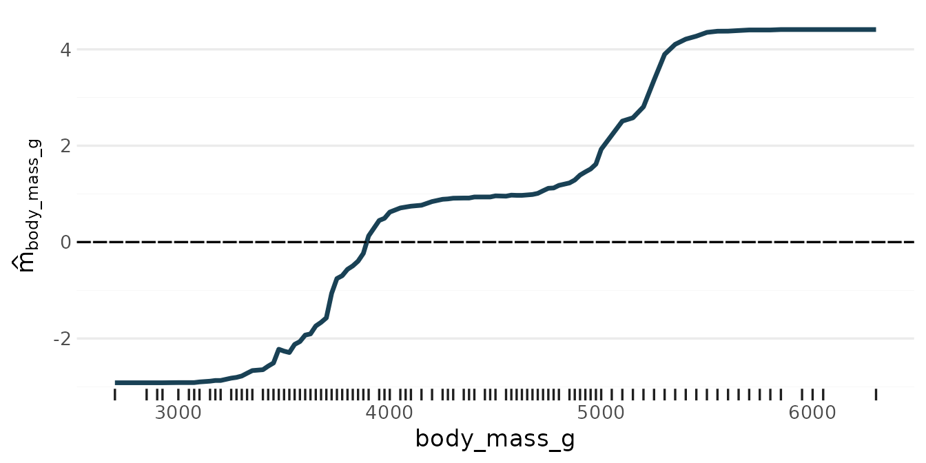

Three or more classes

With more classes, the model has one score per class, and the scores sum to 0. The difference of two classes’ scores is the log-odds of one class against the other. Every component has one column per class:

set.seed(1)
by_species <- rpf(species ~ ., data = penguins, nthreads = 2)
by_species
#> ── Random Planted Forest model ─────────────────────────────────────────────────
#> Classification (logit loss), 3 classes: Adelie, Chinstrap, Gentoo. Scores = intercept + the sum of 2 components.
#> Intercept per class: Adelie   9.01628, Chinstrap -12.59247, Gentoo   3.57619
#> 
#> Components (largest first), importance = share of the variance of the scores (centred across the classes) on the training rows:
#>  component      importance
#>  island         95%       
#>  bill_length_mm 4.1%      
#> 
#> How it was chosen:
#>   The forest: 200 tree families of 30 splits (chosen out of bag; growing stopped at 42).
#>   From the forest's 60 nonzero components (purified): those with a share of at least 10% of the forest's Var(prediction), each with one coefficient, fitted out of bag (rule R).
#>   Rule and threshold chosen by out-of-bag error (1-SE rule; 5 folds, seed 682372961) among 16 candidates.
#>   Left out: 58 components, shares together 14% (largest bill_depth_mm, 5.6%).
predict(by_species, penguins[c(1, 200, 300), ])
#> # A tibble: 3 × 3
#>   .pred_Adelie .pred_Chinstrap .pred_Gentoo
#>          <dbl>           <dbl>        <dbl>
#> 1     1.000          1.65 e-20     2.36e- 4
#> 2     0.00612        5.04 e-17     9.94e- 1
#> 3     0.000245       1.000e+ 0     1.88e-10

comp3 <- predict_components(by_species, penguins)
comp3$target_levels
#> [1] "Adelie"    "Chinstrap" "Gentoo"
names(comp3$m)[1:6]
#> [1] "bill_length_mm__class:Adelie"    "bill_length_mm__class:Chinstrap"
#> [3] "bill_length_mm__class:Gentoo"    "island__class:Adelie"           
#> [5] "island__class:Chinstrap"         "island__class:Gentoo"
comp3$intercept
#>     Adelie  Chinstrap     Gentoo 
#>   9.016282 -12.592471   3.576189

The columns are named <component>__class:<level>, one for each of Adelie, Chinstrap and Gentoo. A positive contribution moves a penguin towards that class, a negative one away from it, and no class is singled out as a reference. A component is kept or dropped for all classes together: its size is its variance summed over the classes’ scores, centred across the classes. glex draws one panel per score:

plot(comp3, "bill_length_mm")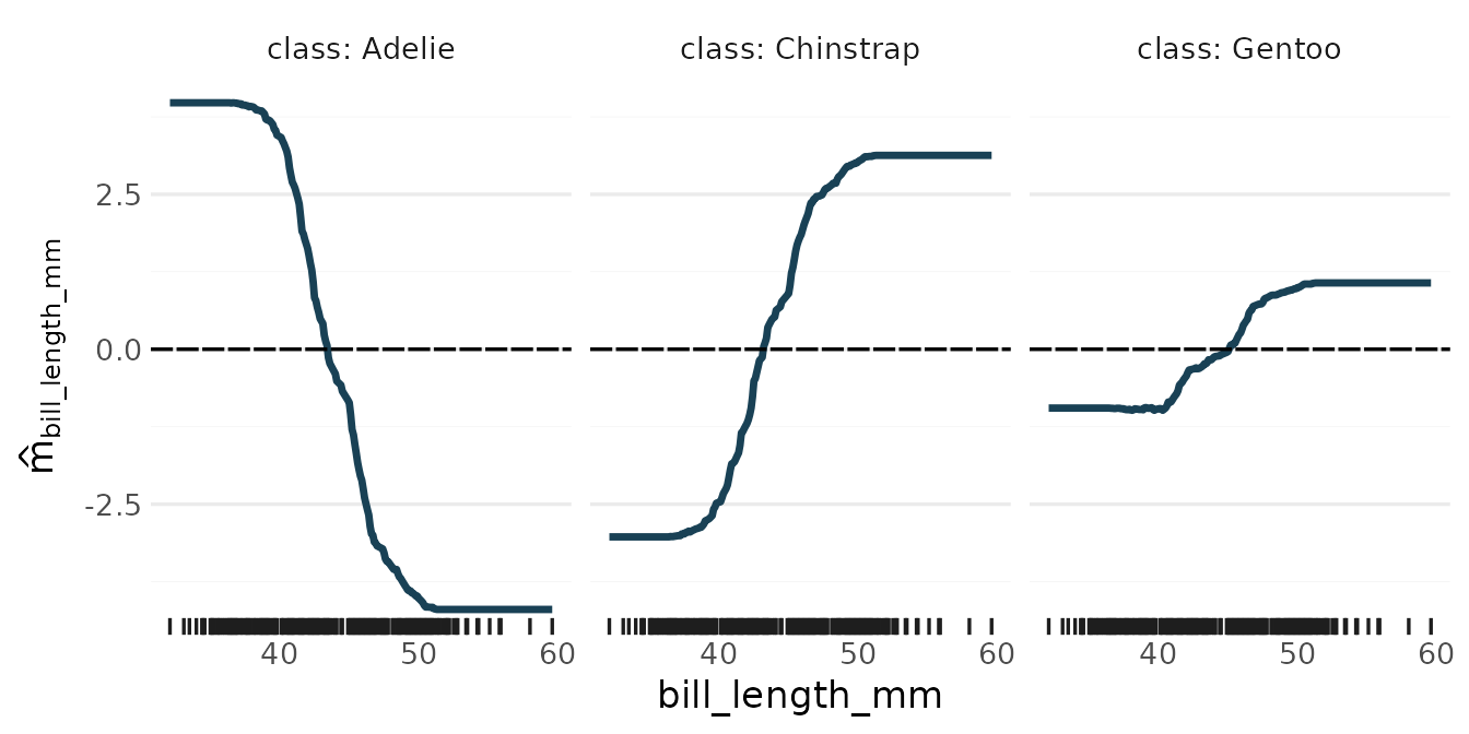

How the choices are scored

Every out-of-bag choice, of the number of splits and of the pruning, is scored by the loss’s own criterion, corrected for the number of out-of-bag families as for regression:

• for the losses that give probabilities, the log-loss of the probabilities predict(type = "prob") returns;
• for loss = "L1" and "L2", which fit class indicators directly, the squared error of the scores summed over the classes (the Brier score).

The losses

loss chooses how the families fit the classes:

• "logit" (the default) and "exponential" fit scores on the link scale, and predict(type = "prob") returns their softmax, so the probabilities are proper. With two classes there is one score, the log-odds of the second class. With more, both have one score per class, summing to 0, so the link predictions and the components have one column per class. "logit" is the multinomial log-likelihood and "exponential" the multiclass exponential loss SAMME.
• "L1" and "L2" fit 0/1 class indicators directly, as regression would; their scores are not probabilities, and type = "prob" truncates them to [0, 1].

A step, and the pseudo-row

Every split moves the scores of the rows of each of its two new leaves by one step. For "exponential" and "logit", the step minimises the leaf’s penalised loss: the loss of its rows plus that of one imaginary row, the pseudo-row, split evenly over the classes and placed at the score the leaf has now. The pseudo-row says “stay where you are”, so it pulls every step towards no change, and more so the fewer rows the leaf has.

Two things follow:

• A pure leaf stops at a finite level. If all rows of a leaf have one class, the loss of its rows alone falls forever as its score grows, and an unpenalised step would push the score to infinity. The pseudo-row, which holds a share of the other classes, stops it: with two classes a pure leaf of n rows goes to about log(2n + 1) and then stays there.
• A pure split or a repeat gains nothing. A split is scored by what its two leaves’ steps gain over the step the parent leaf would make by itself, and each new leaf pays for its own pseudo-row. Splitting a pure leaf cannot separate anything, and repeating a split whose leaves are already at their best level cannot improve them, so both score no gain and are not made. A round in which no candidate gains makes no split (it still counts towards n_splits).

The table shows the score of a point in a pure region as one tree family grows: the two classes are separated by x1 > 0.5, and x2 is noise. The fits leave out the forest’s level (below), so that the table shows the steps alone.

old <- options(randomPlantedForest.level = FALSE)
set.seed(1)
n <- 200
sep <- data.frame(x1 = runif(n), x2 = runif(n))
sep$y <- factor(ifelse(sep$x1 > 0.5, "b", "a"))

rounds <- c(5, 10, 30, 100, 300)
score_after <- function(loss, k) {
  set.seed(3)
  f <- rpf(y ~ ., data = sep, loss = loss, n_families = 1, n_splits = k, prune = FALSE)
  c(score = predict(f, data.frame(x1 = 0.9, x2 = 0.5), type = "link")$.pred,
    leaves = nrow(rpf_boxes(f)) - 1)
}
pure <- data.frame(
  rounds = rounds,
  t(sapply(rounds, function(k) score_after("exponential", k))),
  t(sapply(rounds, function(k) score_after("logit", k)))
)
names(pure) <- c("rounds", "exponential score", "exponential leaves", "logit score", "logit leaves")
options(old)
pure
#>   rounds exponential score exponential leaves logit score logit leaves
#> 1      5          1.036092                  2    1.036092            2
#> 2     10          5.200472                  6    5.219555            6
#> 3     30          5.876469                 11    5.070276           13
#> 4    100          6.439066                 13    5.070276           13
#> 5    300          6.439066                 13    5.070276           13

The score stays at its level from the first rounds on, and the family soon stops adding leaves: no candidate gains any more. So a fixed, large n_splits does not make the model overconfident.

exact_step

"exponential"’s step has a closed form, so it is exact. "logit" scores the candidates by the second-order (Newton) gain of its penalised loss. With exact_step = TRUE (the default), the chosen split’s two leaves then get the exact minimisers, by Newton’s method on their rows; exact_step = FALSE keeps the one Newton step, which is a little faster. The search is the same either way, and exact_step does not change "exponential" fits.

The level

The tree families are averaged on the score scale. Where they disagree, the probability of their mean score is not the mean of their probabilities: for a class rarer than 1/2 it is lower, and the more splits the families make, the more they disagree. So after the fit, a forest with "logit" or "exponential" gets one constant per score column, its level: the intercept that makes every class’s mean out-of-bag probability equal to its frequency in the training rows (the maximum-likelihood intercept given the forest’s out-of-bag scores). The level is part of the forest’s intercept, so the components and the purified forest include it, and the pruning starts from the forest with it. $level holds it, print() shows it, and options(randomPlantedForest.level = FALSE) fits without it.