Getting Started with randomPlantedForest

randomPlantedForest implements Random Planted Forest (Hiabu, Mammen & Meyer), a directly interpretable tree ensemble. Its defining feature is that the maximum order of interaction between predictors can be bounded via max_interaction: the fitted model then decomposes exactly into main effects, two-way interactions, and so on, a functional ANOVA decomposition, with no post-hoc approximation needed.

library(randomPlantedForest)

Fitting a regression forest

To see what the model recovers, we simulate data where the true components are known. The outcome depends on x1, x2 and x3 through main effects of different shapes and on x1 and x2 jointly through a product interaction with x4 having no effect at all:

$$y = 1 + \sin(\pi x_1) + 2\left(x_2^2 - \tfrac{1}{3}\right) + \tfrac{x_3}{2} + 2 x_1 x_2 + \varepsilon$$

With uniform predictors on $[-1, 1]$, each term has mean zero and the interaction has no main-effect part, so the terms are exactly the components the model is meant to estimate.

set.seed(1)
n <- 1000
sim <- data.frame(
  x1 = runif(n, -1, 1),
  x2 = runif(n, -1, 1),
  x3 = runif(n, -1, 1),
  x4 = runif(n, -1, 1)
)
true_effects <- list(
  x1 = function(x) sin(pi * x),
  x2 = function(x) 2 * (x^2 - 1 / 3),
  x3 = function(x) x / 2
)
sim$y <- 1 +
  true_effects$x1(sim$x1) +
  true_effects$x2(sim$x2) +
  true_effects$x3(sim$x3) +
  2 * sim$x1 * sim$x2 +
  rnorm(n, sd = 0.3)

rpfit <- rpf(y ~ ., data = sim, max_interaction = 2, ntrees = 50)
rpfit
#> ── Regression Random Planted Forest ────────────────────────────────────────────
#> Formula: `y ~ .`
#> 50 tree families with 30 splits each on 4 predictors, interactions to degree 2.
#> ℹ Forest is not purified.
#> 
#> ── Tree growing 
#>    split_structure: leaves
#>          split_try: 10
#>              t_try: 0.4
#>     max_candidates: 50
#>   split_decay_rate: 0.1
#>      delete_leaves: TRUE
#> 
#> ℹ Fit using 1 thread, also the default for `predict()` and `purify()`.

max_interaction = 2 restricts the forest to main effects and two-way interactions. This is the central tuning choice of the method: lower values give a more interpretable, more constrained model, while max_interaction = 0 allows interactions of any order. ntrees sets the number of tree families in the ensemble.

Prediction works as usual:

predict(rpfit, new_data = head(sim))
#> # A tibble: 6 × 1
#>     .pred
#>     <dbl>
#> 1 -0.217 
#> 2  0.0562
#> 3  1.27  
#> 4  3.83  
#> 5  1.17  
#> 6  0.955

Note that rpf() does not handle missing values: rows containing NA must be imputed or removed beforehand (see the recipes section below for one way to do this as part of the model specification).

Decomposing predictions

Because the interaction order is bounded, the prediction function is a sum of low-dimensional components:

$$\hat{m}(x) = \hat{m}_0 + \sum_k \hat{m}_k(x_k) + \sum_{k < l} \hat{m}_{kl}(x_k, x_l)$$

predict_components() returns exactly this decomposition: an intercept and one column per main effect and interaction term, evaluated on the supplied data. The forest is purified internally to make the decomposition unique, which is why the print method above reports the purification state.

components <- predict_components(rpfit, new_data = sim)

components$intercept
#> [1] 0.9862177
names(components$m)
#>  [1] "x1"    "x2"    "x3"    "x4"    "x1:x2" "x1:x3" "x1:x4" "x2:x3" "x2:x4"
#> [10] "x3:x4"

The components sum exactly to the model prediction:

pred_sum <- components$intercept + rowSums(components$m)
pred_direct <- predict(rpfit, new_data = sim)$.pred

all.equal(pred_sum, pred_direct)
#> [1] TRUE

Each column of components$m is the isolated contribution of one predictor (or one pair) to the prediction, on the scale of the outcome. Their standard deviations give a simple importance measure: the three main effects and the x1:x2 interaction dominate, while x4 and the other interactions are close to zero, as they should be.

round(sort(sapply(components$m, sd), decreasing = TRUE), 3)
#> x1:x2    x1    x2    x3 x2:x3 x1:x3    x4 x1:x4 x2:x4 x3:x4 
#> 0.656 0.655 0.573 0.258 0.026 0.007 0.000 0.000 0.000 0.000

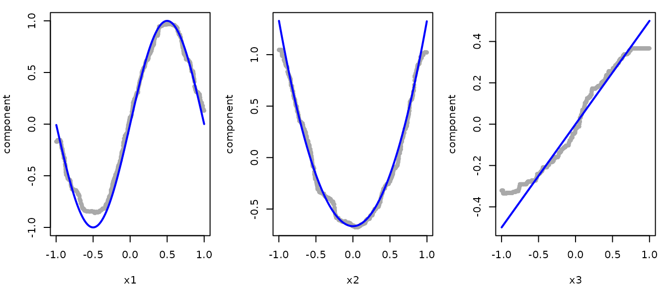
The estimated main effects follow the true functions (blue lines). As with any tree-based model, they flatten out towards the edges of the data, where few observations are available to determine them.

op <- par(mfrow = c(1, 3), mar = c(4, 4, 1, 1))
for (v in names(true_effects)) {
  ylim <- range(components$m[[v]], true_effects[[v]](sim[[v]]))
  plot(
    sim[[v]],
    components$m[[v]],
    pch = 20,
    col = "darkgray",
    ylim = ylim,
    xlab = v,
    ylab = "component"
  )
  curve(true_effects[[v]](x), add = TRUE, lwd = 2, col = "blue")
}

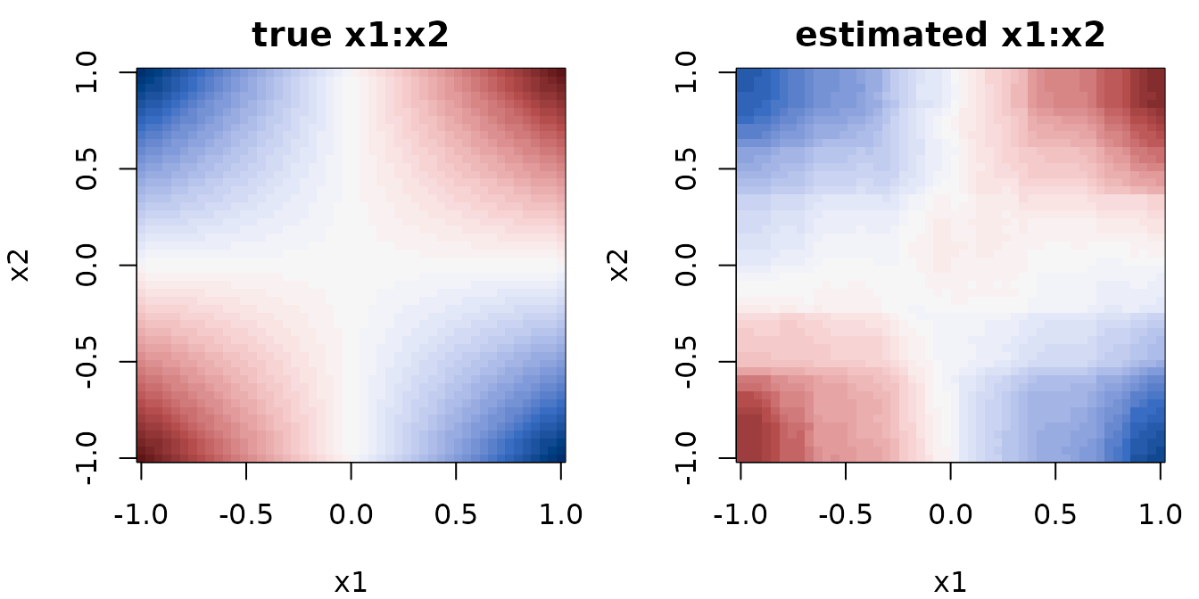
par(op)

The interaction is a function of two variables, so it is shown as a heatmap. We evaluate the estimated x1:x2 component on a grid. Note x3 and x4 must be present in the new data but do not affect this component.

grid_points <- seq(-1, 1, length.out = 50)
grid <- expand.grid(x1 = grid_points, x2 = grid_points, x3 = 0, x4 = 0)
estimated <- predict_components(rpfit, new_data = grid, predictors = c("x1", "x2"))$m[["x1:x2"]]

surfaces <- list(
  true = outer(grid_points, grid_points, function(x1, x2) 2 * x1 * x2),
  estimated = matrix(estimated, nrow = length(grid_points))
)
zlim <- c(-1, 1) * max(abs(unlist(surfaces)))

op <- par(mfrow = c(1, 2), mar = c(4, 4, 2, 1))
for (s in names(surfaces)) {
  image(
    grid_points,
    grid_points,
    surfaces[[s]],
    zlim = zlim,
    col = hcl.colors(51, "Blue-Red 3"),
    xlab = "x1",
    ylab = "x2",
    main = paste(s, "x1:x2")
  )
}

par(op)

The plots above are drawn manually from predict_components() for illustration. The glex package provides ggplot2 versions of them: glex() computes the decomposition for a fitted rpf object, and plot_main_effect() and plot_twoway_effects() draw main effects and two-way interactions.

Classification

For a factor outcome, rpf() automatically fits a classification forest. We illustrate with the penguins data from palmerpenguins, removing missing values first.

Binary

penguins <- na.omit(palmerpenguins::penguins)

rpfit_sex <- rpf(sex ~ ., data = penguins, ntrees = 50)

predict(rpfit_sex, head(penguins), type = "prob")
#> # A tibble: 6 × 2
#>   .pred_female .pred_male
#>          <dbl>      <dbl>
#> 1       0.0591    0.941  
#> 2       0.806     0.194  
#> 3       0.995     0.00546
#> 4       0.998     0.00219
#> 5       0.0243    0.976  
#> 6       0.992     0.00801
predict(rpfit_sex, head(penguins), type = "class")
#> # A tibble: 6 × 1
#>   .pred_class
#>   <fct>      
#> 1 male       
#> 2 female     
#> 3 female     
#> 4 female     
#> 5 male       
#> 6 female

With the default loss = "exponential" (or "logit"), type = "link" additionally gives raw predictions on the log-odds scale.

Multiclass

Multiclass classification works the same way: probability predictions contain one column per class:

rpfit_species <- rpf(species ~ ., data = penguins, ntrees = 50)

predict(rpfit_species, head(penguins), type = "prob")
#> # A tibble: 6 × 3
#>   .pred_Adelie .pred_Chinstrap .pred_Gentoo
#>          <dbl>           <dbl>        <dbl>
#> 1        1.000   0.00000000457     1.35e-11
#> 2        1.000   0.0000000237      5.63e-11
#> 3        1.000   0.0000000217      3.63e-11
#> 4        1.000   0.00000000188     7.16e-12
#> 5        1.000   0.00000000200     8.66e-12
#> 6        1.000   0.0000000225      4.10e-11
predict(rpfit_species, head(penguins), type = "class")
#> # A tibble: 6 × 1
#>   .pred_class
#>   <fct>      
#> 1 Adelie     
#> 2 Adelie     
#> 3 Adelie     
#> 4 Adelie     
#> 5 Adelie     
#> 6 Adelie

The default loss for classification is "exponential", which gives proper probability estimates. "logit" gives similar results but is slower, while "L1" and "L2" fit class indicators directly and do not yield proper probabilities. Note that with loss = "logit", multiclass models are fit on a reference-class (log-odds) scale, so link predictions and components have one column less than there are classes: see ?predict.rpf for details.

Using recipes

rpf() also accepts a recipes recipe in place of a formula, so preprocessing can be bundled with the model specification. This makes it easy to add preprocessing steps, such as imputing missing values, which rpf() itself does not accept:

library(recipes)

# rows with a missing outcome still need to be dropped by hand
peng_raw <- subset(palmerpenguins::penguins, !is.na(body_mass_g))

rec <- recipe(body_mass_g ~ ., data = peng_raw) |>
  step_impute_median(all_numeric_predictors()) |>
  step_impute_mode(all_nominal_predictors())

rpfit_rec <- rpf(rec, data = peng_raw, ntrees = 50)

predict(rpfit_rec, head(peng_raw))
#> # A tibble: 6 × 1
#>   .pred
#>   <dbl>
#> 1 3801.
#> 2 3491.
#> 3 3572.
#> 4 3482.
#> 5 4006.
#> 6 3422.

The preprocessing steps are stored with the model and applied automatically in predict().

Saving and restoring models

An rpf object holds its forest in an external pointer to a C++ object, which saveRDS() cannot preserve, meaning that a naively saved and restored model is not usable:

tmp <- tempfile(fileext = ".rds")
saveRDS(rpfit, tmp)
broken <- readRDS(tmp)

rpf_is_valid(broken)
#> [1] FALSE
predict(broken, head(sim))
#> Error in `predict()`:
#> ! The C++ forest behind this <rpf> object is gone.
#> ℹ Most likely it was saved with `saveRDS()` and restored with `readRDS()`.
#> ℹ Use `blob <- rpf_marshal(x)` before saving and `rpf_unmarshal(blob)` after
#>   loading, see `?rpf_marshal()`.

Use rpf_marshal() to convert the model into a plain R list before saving, and rpf_unmarshal() after loading:

saveRDS(rpf_marshal(rpfit), tmp)
restored <- rpf_unmarshal(readRDS(tmp))

all.equal(
  predict(restored, head(sim)),
  predict(rpfit, head(sim))
)
#> [1] TRUE

Alternatively, a bundle method wrapping the same mechanism is available via bundle::bundle() and bundle::unbundle().