How the forest is grown

A random planted forest is an average of tree families, each grown on a bootstrap sample of the training rows. What makes it interpretable is the family: a sum of trees, each of which splits on its own small set of predictors. This article shows one family as it grows, then the settings that control the growth.

library(randomPlantedForest)

Data

The outcome depends on x1, x2 and x3 through main effects of different shapes, and on x1 and x2 jointly through a product; x4 has no effect.

$$y = 1 + \sin(\pi x_1) + 2\left(x_2^2 - \tfrac{1}{3}\right) + \tfrac{x_3}{2} + 2 x_1 x_2 + \varepsilon$$

set.seed(1)
n <- 1000
sim <- data.frame(
  x1 = runif(n, -1, 1),
  x2 = runif(n, -1, 1),
  x3 = runif(n, -1, 1),
  x4 = runif(n, -1, 1)
)
sim$y <- 1 + sin(pi * sim$x1) + 2 * (sim$x2^2 - 1 / 3) + sim$x3 / 2 +
  2 * sim$x1 * sim$x2 + rnorm(n, sd = 0.3)

One tree family

To look at a family, we fit a forest of a single family with 10 splits, of at most two predictors per tree, and keep the forest (prune = FALSE):

set.seed(6)
small <- rpf(y ~ ., data = sim, max_interaction = 2, n_families = 1, n_splits = 10, prune = FALSE)
plot(small)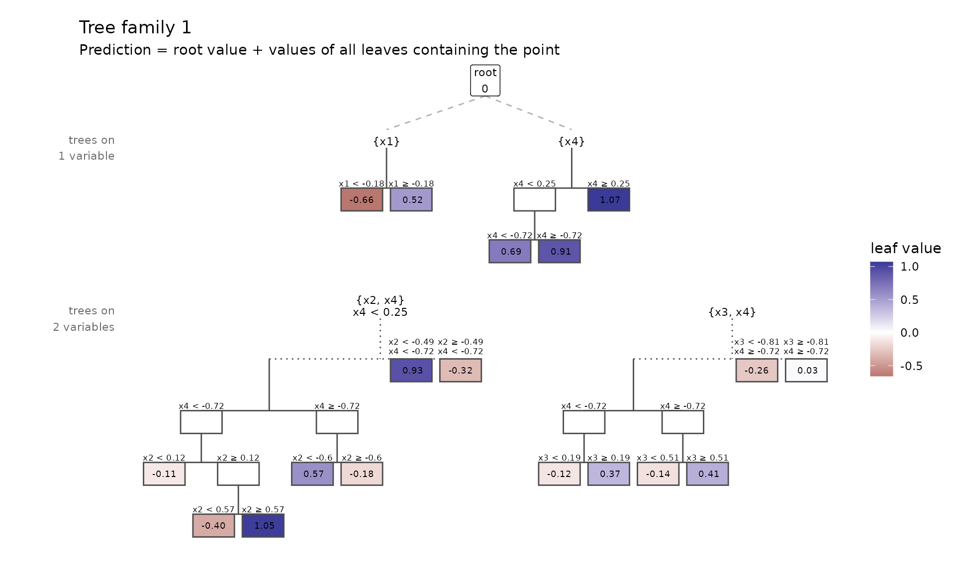

The family starts with the root, a single leaf of value 0 that covers all the data. Every split takes one leaf of one tree, a predictor and a threshold, and fits the two halves to what the family does not yet explain (for regression, the residuals):

• If the tree already splits on that predictor, the leaf is replaced by its two halves.
• If it does not, the two halves go to the tree on the tree’s predictors plus the new one, which is created if needed, and the leaf stays where it was, so that it can be split again on other predictors.

So the family grows trees on single predictors from the root, trees on pairs from those, and so on. max_interaction caps how many predictors a tree may have. The prediction of the family for a point is the sum of the values of all leaves, in all trees, that contain it; the forest averages the families.

The diagram shows the trees in rows by the number of predictors they split on, with each leaf coloured by its value. plot(type = "boxes") draws the same leaves in the space of the predictors, one panel per tree:

plot(small, type = "boxes")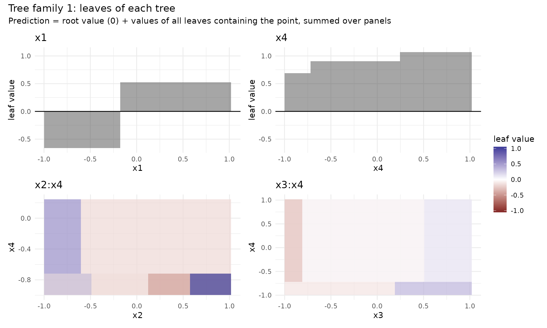

From trees to components

The trees are not yet the components of the model. Leaves of different trees overlap, so an effect can be spread over several trees: the quadratic effect of x2 can sit in the tree on x2 alone, or in the tree on x1 and x2. Purification moves every effect to the lowest-order tree it belongs to, without changing the family’s prediction:

purify(small)
plot(small, type = "boxes")

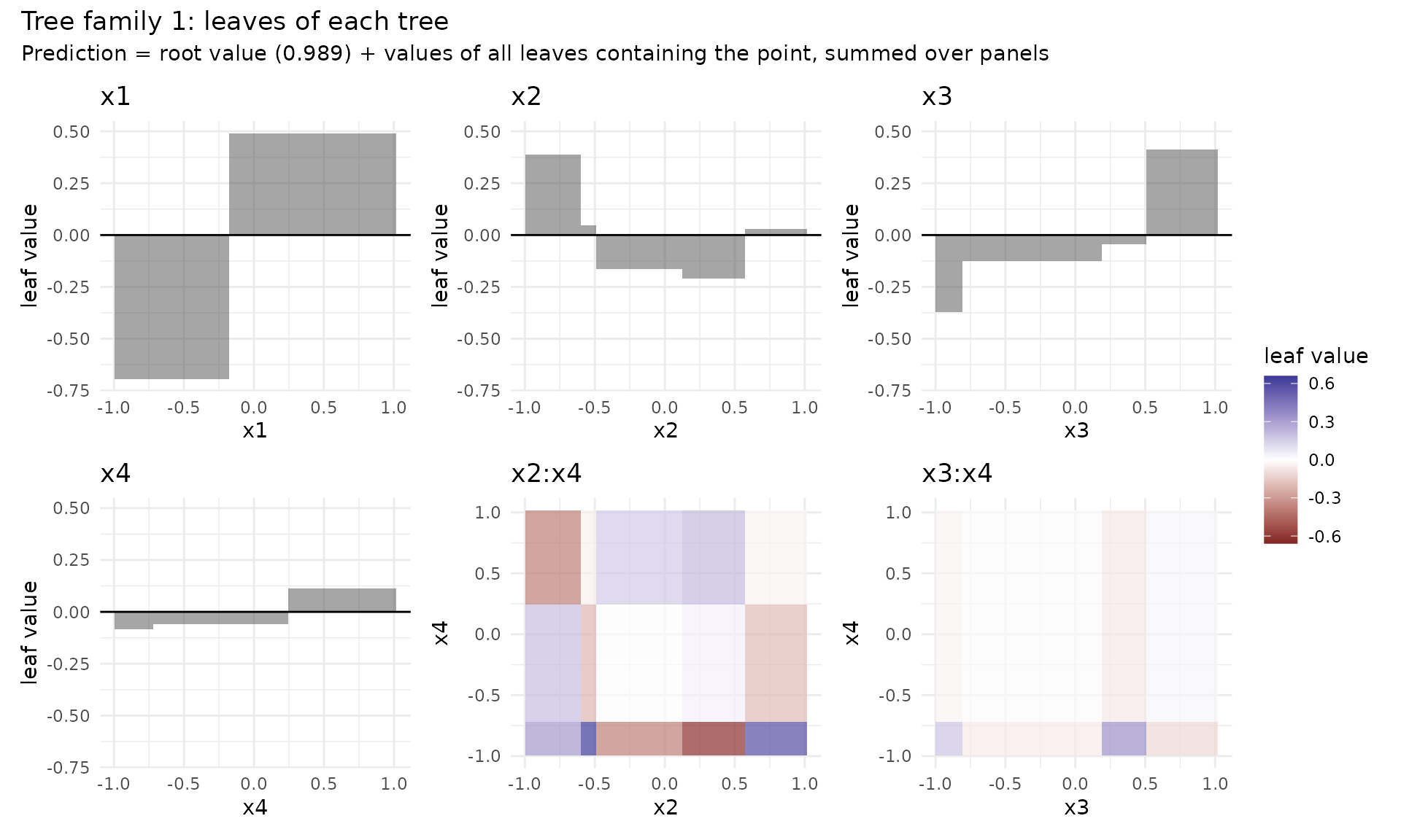
Now each panel is one component of this family, and the root value is its intercept. A family of ten splits is a rough model: it can miss a true effect or grow an interaction the data do not have. The other families, grown on other bootstrap samples with other random draws, do not share these errors. Averaging the components over 200 families, with the number of splits chosen for the data, and pruning the small ones gives the estimates of Reading the model.

max_interaction

max_interaction decides which components the model can have: 1 gives an additive model, 2 adds pairwise interactions, 3 (the default) three-way interactions, and 0 sets no limit. A lower order is easier to read but cannot represent interactions of higher order; a higher one spreads the splits over many more possible components, and costs more time.

To see the difference, we add a three-way interaction to the outcome and fit the default model at each order, then compare the error on new data:

make_data <- function(n) {
  d <- data.frame(matrix(runif(n * 5, -1, 1), ncol = 5, dimnames = list(NULL, paste0("x", 1:5))))
  d$y <- sin(pi * d$x1) + d$x2 + 2 * d$x1 * d$x3 + 3 * d$x2 * d$x3 * d$x4 + rnorm(n, sd = 0.3)
  d
}
set.seed(3)
train <- make_data(1000)
test <- make_data(2000)

rmse <- sapply(1:3, function(order) {
  m <- rpf(y ~ ., data = train, max_interaction = order, n_families = 50, nthreads = 2)
  sqrt(mean((test$y - predict(m, test)$.pred)^2))
})
data.frame(max_interaction = 1:3, test_rmse = round(rmse, 3))
#>   max_interaction test_rmse
#> 1               1     0.957
#> 2               2     0.666
#> 3               3     0.352

The noise has standard deviation 0.3, the lowest error any model can reach. Only order 3 can hold the three-way term.

The split search

Each round of a family’s growth draws some possible splits as candidates, tries a few thresholds for each, and makes the best split among them. Five settings control this search:

• split_structure: what a candidate is (see below).
• share_candidates: the share of all possible splits drawn as candidates each round, at most max_candidates (50).
• n_try_split_points: how many thresholds are tried per candidate.
• split_decay_rate (aging): a possible split that was a candidate but not chosen ages by one; possible splits are drawn with weight exp(-split_decay_rate * age), so the draw moves on to splits not yet tried. 0 draws uniformly.
• min_leaf_rows: the fewest rows of the bootstrap sample on each side of a split, so in every leaf (1, no limit, by default).

The more candidates and thresholds a round tries, the greedier the search. For the default structure, a search that is not very greedy is often better: the default tries 3 thresholds and 10% of the possible splits per round. rpf(tune = TRUE) searches the greediness and min_leaf_rows out of bag for your data (see The number of splits and further tuning).

Split structures

split_structure	a candidate is	its thresholds
"leaf" (default)	a leaf and a predictor	n_try_split_points of the leaf’s distinct values
"leaf_binned"	a leaf and a predictor	boundaries of quantile bins, computed once per predictor; faster on large data
"tree_then_leaf"	a tree and a predictor	n_try_split_points times: a leaf of the tree, drawn by its number of possible thresholds, and one threshold in it
"tree_then_all_leaves"	a tree and a predictor	every leaf of the tree, n_try_split_points thresholds each
"target_tree_then_leaf"	the tree the split grows into	n_try_split_points times: a leaf and predictor, then one threshold

"leaf" is the default and the structure the defaults were chosen for; the others default to 10 thresholds and 40% of the candidates. ?rpf describes each structure in detail.

Constraining interactions

interaction_constraints restricts which predictors may share a tree, as in xgboost: a tree is grown only if its predictors are a subset of one of the given sets.

constrained <- rpf(
  y ~ ., data = sim, interaction_constraints = list(c("x1", "x2"), c("x3", "x4")),
  n_families = 50, nthreads = 2
)
constrained$components[, c("component", "share", "kept")]
#>   component        share  kept
#> 1        x1 0.3321078983  TRUE
#> 2        x2 0.2575106612  TRUE
#> 3        x3 0.0559141664  TRUE
#> 4        x4 0.0001174298 FALSE
#> 5     x1:x2 0.3411360769  TRUE
#> 6     x3:x4 0.0002180949 FALSE

The forest has no component that joins a predictor of one set with one of the other, such as x1:x3; of the components it has, pruning keeps those large enough.

Randomness and reproducibility

A family’s randomness is its bootstrap sample and its draws of candidates and thresholds. With the same seed, rpf() gives the same forest on the same platform, with any number of threads. Another platform can give another forest for the same seed, because the C++ standard libraries draw random integers differently.

The candidates of "leaf" are drawn by a fast draw that keeps the weights in a tree between rounds.