Categorical features: native factors, one-hot groups and semantic groups

library(glex)
library(xgboost)
set.seed(1)

A categorical predictor can reach xgboost in two ways, and glex handles both:

Native factors (xgboost >= 3.0): fit on a data.frame with factor columns. The trees split on sets of levels, and the decomposition treats the factor as one feature from the start.
Dummy encoding via model.matrix(): the classic route, and the only one for models fit before native support. The decomposition then sees one feature per level, and group_components() re-assembles the factor afterwards.

group_components() also serves a third purpose: treating any set of features as one, e.g. a block of related measurements.

The built-in bike data has a four-level season factor alongside numeric predictors:

data(bike, package = "glex")
x_df <- as.data.frame(bike[, c("season", "hr", "temp", "hum")])
str(x_df)
#> 'data.frame':    8645 obs. of  4 variables:
#>  $ season: Factor w/ 4 levels "Winter","Spring",..: 1 1 1 1 1 1 1 1 1 1 ...
#>  $ hr    : num  0 1 2 3 4 5 6 7 8 9 ...
#>  $ temp  : num  0.24 0.22 0.22 0.24 0.24 0.24 0.22 0.2 0.24 0.32 ...
#>  $ hum   : num  0.81 0.8 0.8 0.75 0.75 0.75 0.8 0.86 0.75 0.76 ...

Native factors

With a data.frame input, xgboost() treats factor columns as categorical. Pass the same data.frame to glex(); the factor levels must match the training data in order, as for predict().

xg_native <- xgboost(
  x_df,
  bike$bikers,
  nrounds = 50,
  max_depth = 3,
  learning_rate = 0.1,
  nthreads = 2
)
res_native <- glex(xg_native, x_df)
names(res_native$m)
#>  [1] "season"             "hr:season"          "hr:season:temp"    
#>  [4] "season:temp"        "hr"                 "hr:temp"           
#>  [7] "temp"               "hr:hum:season:temp" "hr:hum:season"     
#> [10] "hum:season:temp"    "hum:season"         "hr:hum:temp"       
#> [13] "hr:hum"             "hum:temp"           "hum"

season is one feature: there is a single main effect and single interactions with the numeric predictors. The factor column is kept in $x, so plots treat it as categorical:

plot_main_effect(res_native, "season")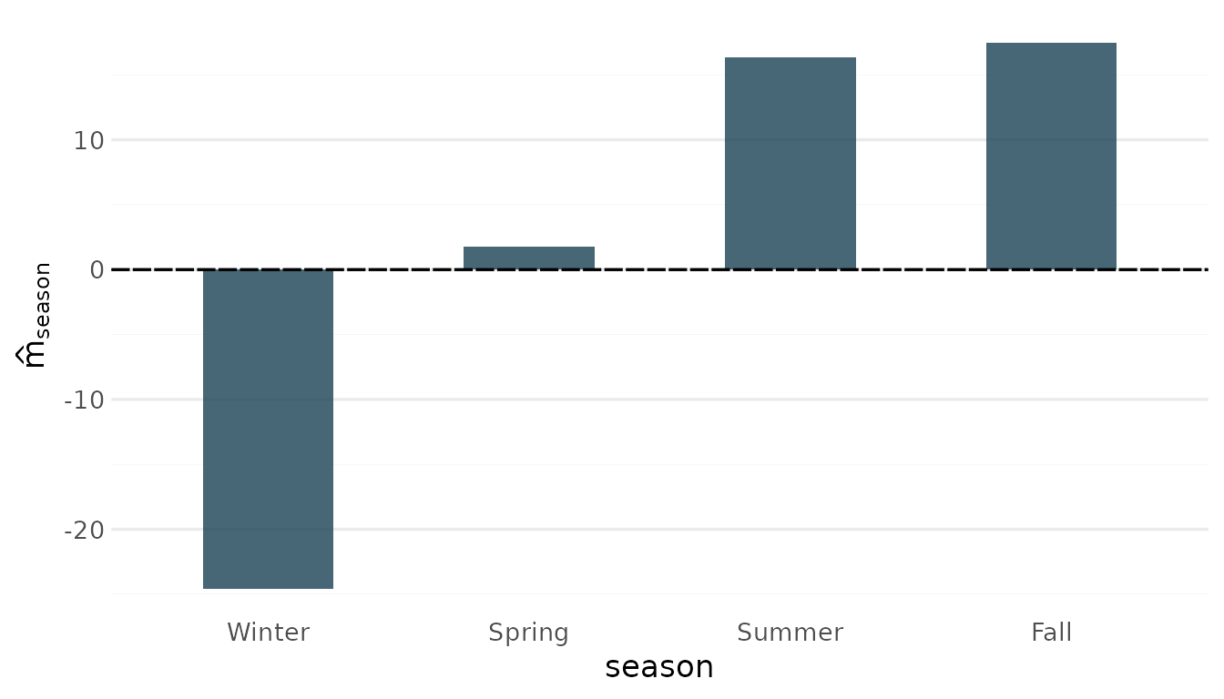

plot_twoway_effects(res_native, c("season", "temp"))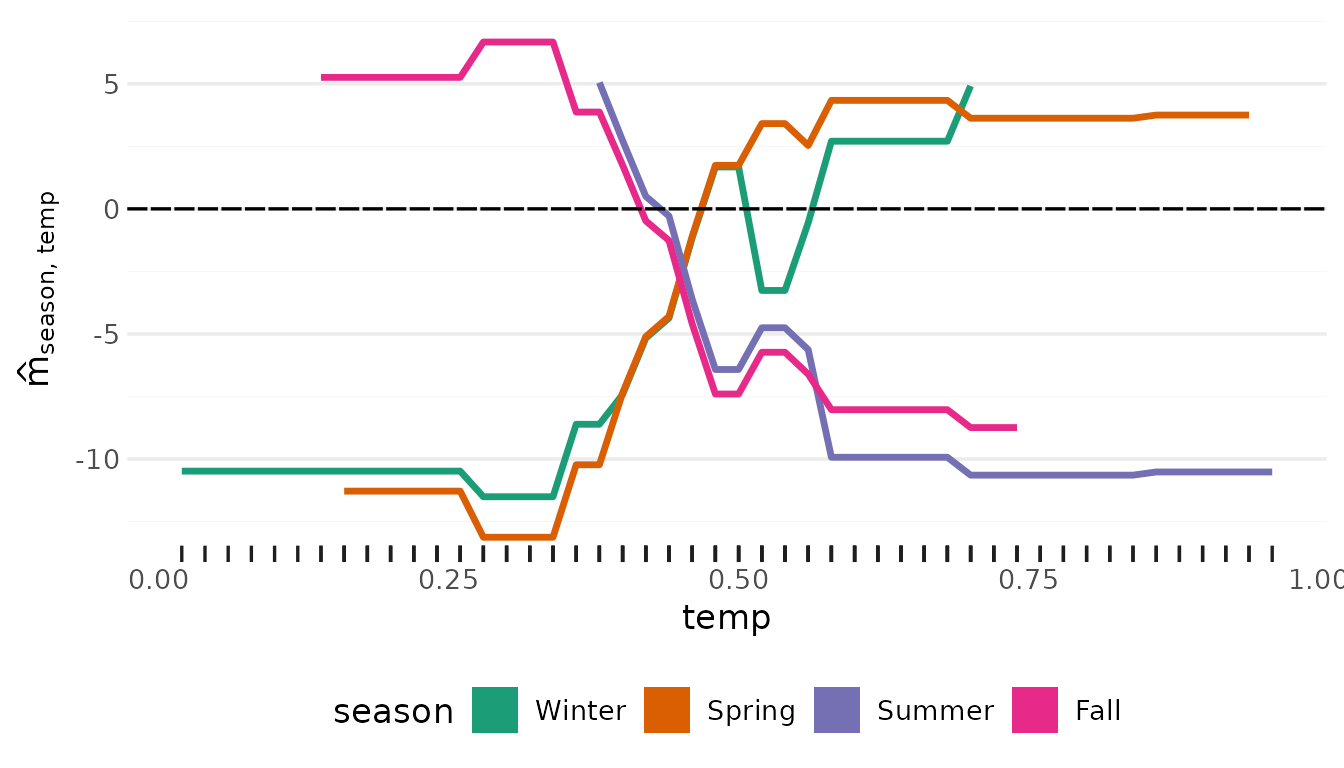

Dummy encoding fragments the decomposition

Encoding season with model.matrix() gives one column per level. The decomposition then treats every dummy column as a feature of its own: the effect of the factor is smeared across its dummies and their mutual “interactions”, which are artifacts of the encoding rather than anything about the data.

x <- cbind(
  model.matrix(~ season - 1, bike),
  as.matrix(bike[, c("hr", "temp", "hum")])
)
colnames(x)
#> [1] "seasonWinter" "seasonSpring" "seasonSummer" "seasonFall"   "hr"          
#> [6] "temp"         "hum"

xg <- xgb.train(
  params = xgb.params(max_depth = 3, learning_rate = 0.1, nthread = 2),
  data = xgb.DMatrix(x, label = bike$bikers, nthread = 2),
  nrounds = 50
)
res <- glex(xg, x)
ncol(res$m)
#> [1] 47

Among these terms are things like seasonFall:seasonWinter, an “interaction” between two levels of the same factor:

head(sort(colMeans(abs(as.matrix(res$m))), decreasing = TRUE), 10)
#>              hr            temp         hr:temp             hum    seasonWinter 
#>       65.597247       35.139222       16.901747       14.016117       10.907372 
#>          hr:hum      seasonFall hr:seasonWinter        hum:temp seasonFall:temp 
#>        8.785011        6.212056        4.371334        3.667917        2.827076

Re-assembling the factor with `group_components()`

group_components() aggregates all terms feature-wise: terms involving only season dummies become the season main effect, terms mixing a dummy with hr become the season:hr interaction, and so on. Because the decomposition is additive, this is exact.

dummy_groups() builds the required groups list from the un-encoded data, matching the model.matrix() naming convention by default. bike carries further factors (mnth, workingday, weathersit) that we did not encode into x; dummy_groups() reports them and moves on:

dummy_groups(res, bike)
#> No encoded columns found for: mnth, workingday, weathersit. If these were encoded, pass a `naming` function matching the column names in `object$x`.
#> $season
#> [1] "seasonWinter" "seasonSpring" "seasonSummer" "seasonFall"
grouped <- group_components(res, dummy_groups(res, bike))
#> No encoded columns found for: mnth, workingday, weathersit. If these were encoded, pass a `naming` function matching the column names in `object$x`.
names(grouped$m)
#>  [1] "season"             "hr:season"          "hr:season:temp"    
#>  [4] "season:temp"        "hr"                 "hr:temp"           
#>  [7] "temp"               "hr:hum:season:temp" "hr:hum:season"     
#> [10] "hum:season:temp"    "hum:season"         "hr:hum:temp"       
#> [13] "hr:hum"             "hum:temp"           "hum"

The components still sum to the model prediction, and the SHAP value of season is the sum of its dummies’ SHAP values, so the efficiency property is preserved:

all.equal(rowSums(grouped$m), rowSums(res$m))
#> [1] TRUE
all.equal(
  grouped$shap$season,
  rowSums(as.matrix(res$shap[, startsWith(names(res$shap), "season"), with = FALSE]))
)
#> [1] TRUE

Since the grouped columns of x form a one-hot encoding, group_components() reconstructs the factor, and the plot functions work as for the native model:

plot_main_effect(grouped, "season")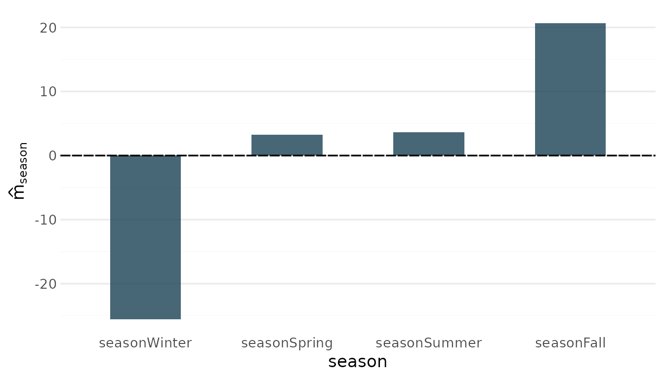

plot_twoway_effects(grouped, c("season", "temp"))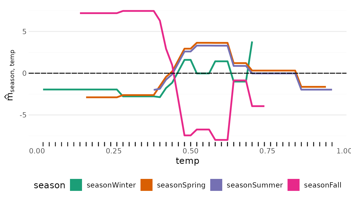

Both routes end with season as one feature, but they explain different models: native categorical splits partition the levels freely, while a dummy split isolates one level at a time. Grouping is an exact regrouping of the dummy model’s decomposition, not an approximation of the native one.

Other encoding schemes

If the dummy columns are not named in model.matrix() style, pass a naming function of (feature, levels) that reproduces the column names the model was trained with:

dummy_groups(
  res,
  bike,
  naming = function(feature, levels) paste(feature, levels, sep = "_")
)

dummy_groups() only returns columns that actually exist in object$x, so a dropped reference level (treatment coding via ~ season) is skipped automatically; the reconstructed factor then shows a "(base)" level for observations of the reference category.

Semantic groups

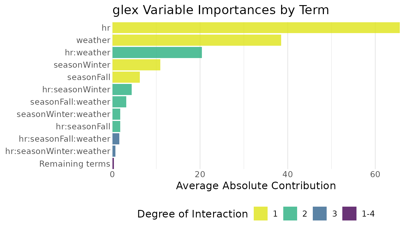
Grouping is not limited to dummy encodings. Any set of features can be treated as one, for example a “weather” block, which in higher-dimensional settings might be a group of anthropometrics, demographics or biomarkers:

weather <- group_components(res, groups = list(weather = c("temp", "hum")))
head(sort(colMeans(abs(as.matrix(weather$m))), decreasing = TRUE), 10)
#>                    hr               weather            hr:weather 
#>             65.597247             38.517036             20.414133 
#>          seasonWinter            seasonFall       hr:seasonWinter 
#>             10.907372              6.212056              4.371334 
#>    seasonFall:weather  seasonWinter:weather         hr:seasonFall 
#>              3.144545              1.799806              1.747389 
#> hr:seasonFall:weather 
#>              1.536791

For such groups no single x value exists, so weather$x$weather is NA and the effect plots are not available for that group, but term importances and SHAP values aggregate as usual:

library(ggplot2)
autoplot(glex_vi(weather), threshold = 0.5)

Native factors

Dummy encoding fragments the decomposition

Re-assembling the factor with group_components()

Other encoding schemes

Semantic groups

Re-assembling the factor with `group_components()`